Revisiting Deep Regression on Tabular Data: The Limits of Loss Functions and Global Early Stopping

Yandex Research finds quantile loss outperforms MSE and exposes systematic flaws of global early stopping on heteroskedastic tabular data.
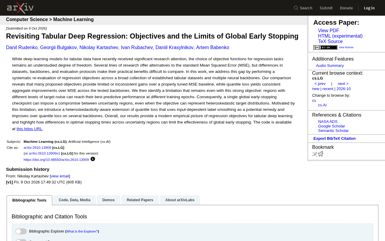
This work from Yandex Research systematically re-evaluates objective function choices for tabular deep regression. It finds that a well-tuned MSE baseline remains competitive and many proposed alternatives offer limited gains, while quantile loss is one of the few options that consistently outperforms MSE across multiple backbones. More critically, the study identifies a previously overlooked training challenge: data regions with different noise levels reach their respective optima at different training epochs, forcing traditional global early stopping to compromise across uncertainty regions. The researchers propose a heteroskedasticity-aware quantile loss extension using input-dependent label smoothing to mitigate this issue, validated across multiple backbone experiments. Code is open-sourced on GitHub.
Deep learning on tabular data has become a hot research topic in recent years, yet the choice of objective function for regression tasks has remained a largely overlooked dimension. Most work defaults to mean squared error (MSE), while empirical comparisons of alternative objectives are fragmented across different datasets, backbone architectures, and evaluation protocols. This work from Yandex Research systematically re-evaluates objective functions for tabular regression and sheds light on a previously underappreciated training challenge — the inherent limitations of global early stopping.
Is MSE Really That Weak?
The research community has proposed multiple lines of work aimed at improving upon MSE, yet their conclusions often contradict one another across different experimental settings, leaving practitioners with little actionable guidance. This study conducts a unified, head-to-head comparison across a broad set of well-established tabular datasets and multiple neural network backbones, aiming to establish a modern, comparable empirical picture.
The conclusion is illuminating: many proposed objective functions show limited or inconsistent gains over a well-tuned MSE baseline. In other words, when MSE is taken seriously and its hyperparameters are carefully tuned, it remains a formidable competitor. This serves as a reminder that when reporting the superiority of a new method, the baseline must itself be sufficiently strong — otherwise, apparent improvements may simply reflect an under-tuned baseline.
Quantile Loss Stands Out
Among all candidates evaluated, quantile loss demonstrated consistent advantages. The study found that across all tested backbone architectures, quantile loss delivers stable overall performance gains over MSE. Unlike objective functions that only work under specific settings, this cross-backbone consistency makes quantile loss a prioritized choice for tabular regression.
The intuition behind this is that quantile loss naturally captures heteroskedastic target distributions — where different regions of the sample space exhibit different noise levels. This also lays the groundwork for the training challenge uncovered next.
Background: Quantile Loss and Heteroskedasticity Quantile loss (also known as Pinball loss) is the standard loss function in quantile regression, used to estimate the conditional distribution of a target variable at a specific quantile (e.g., the median or 10th percentile). For quantile τ ∈ (0,1), the penalty weight is τ when the prediction underestimates the true value, and 1−τ when it overestimates. At τ=0.5, quantile loss reduces to mean absolute error (MAE). Compared to MSE, quantile loss is more robust to outliers and implicitly captures the asymmetry of prediction errors. Heteroskedasticity refers to non-constant noise variance across different regions of the data — for example, high-value houses tend to have larger absolute prediction errors. MSE implicitly assumes homoskedasticity (constant error variance everywhere), which is often an unrealistic assumption for real-world tabular data. This is precisely why quantile loss achieves more consistent advantages in tabular regression tasks.
The Hidden Compromise of Global Early Stopping
Even with a strong objective function like quantile loss, the research team identified an unavoidable training challenge: regions with different levels of target noise tend to reach their optimal predictive performance at different training epochs.
This means that when we follow the conventional practice of selecting a single global early stopping checkpoint, we are effectively forcing a compromise across regions with different levels of uncertainty. Low-noise regions may require more training to converge to their optimum, while high-noise regions may peak earlier and then begin to overfit. A single global stopping point cannot simultaneously serve both — even if the objective function itself is expressive enough to capture heteroskedastic distributions.
The value of this finding is that it shifts the question from "which loss function to use" to the deeper optimization dynamics of "when to stop training." It demonstrates that the expressiveness of the objective function and the convergence behavior of the training process are two independent dimensions, both of which deserve serious attention.
Background: Early Stopping and Its Global Assumption Early stopping is a standard technique in deep learning to prevent overfitting: during training, a validation metric is continuously monitored, and training is halted when the metric fails to improve for a set number of epochs (patience), after which the model reverts to the historical best checkpoint. The "global" aspect here refers to using a single stopping signal for the entire model, treating all samples uniformly. The implicit assumption of global early stopping is that the model's overall performance on the validation set follows a rise-then-fall trajectory, and that the "optimal convergence moment" is roughly synchronized across all sample regions. However, in heteroskedastic settings, high-noise regions (weak signal, high noise) produce noisy gradient signals, causing the model to saturate or even begin overfitting in those regions earlier. Low-noise regions (clear signal) require more iterations to converge to fine-grained decision boundaries. The training dynamics of these two types of regions are systematically misaligned, meaning that a global early stopping point inevitably sacrifices one at the expense of the other — a mechanism that has rarely been explicitly discussed in prior tabular learning research.
A Heteroskedasticity-Aware Extension of Quantile Loss
Building on these insights, the researchers propose a heteroskedasticity-aware extension of quantile loss. The core idea is to use input-dependent label smoothing as a potential mitigation strategy.
Intuitively, this approach allows the model to adaptively adjust the smoothing intensity based on the noise level of the region where an input resides, thereby partially alleviating the inconsistency in optimal stopping times across different regions. Experiments show that this extension further outperforms vanilla quantile loss across multiple backbone architectures, validating the effectiveness of this approach.
Background: Input-Dependent Label Smoothing Label smoothing was originally a regularization technique in image classification, replacing hard labels (0 or 1) with soft labels (e.g., 0.9 and 0.1/num_classes) to prevent models from becoming overconfident. In regression settings, an analogous idea can be understood as applying a slight "perturbation" or "blurring" to target values, making the training signal smoother and more robust to noisy labels. "Input-dependent" smoothing means the smoothing intensity is no longer a global hyperparameter, but is dynamically determined by the model based on the estimated noise level in the region of the current input sample — applying stronger smoothing in high-noise regions to suppress the impulse to overfit, and maintaining smaller smoothing in low-noise regions to preserve fine-grained fitting capacity. This essentially aligns the model's training behavior with local data characteristics, partially compensating at the loss function level for the inability of global early stopping to treat different regions differently.
Takeaways for Practitioners and Researchers
This work offers several directly actionable recommendations:
- Don't underestimate MSE: Before introducing more complex objective functions, ensure the MSE baseline is thoroughly tuned;
- Try quantile loss first: It provides consistent gains across multiple backbones and is a cost-effective default choice;
- Be wary of the compromise effects of global early stopping: When data exhibits clear heteroskedastic structure, a single stopping point may be suboptimal — exploring region-adaptive training strategies is worthwhile.
The research team has open-sourced the complete codebase at github.com/yandex-research/tabular-regression to facilitate community reproduction and further validation. Overall, this paper not only updates the empirical understanding of objective functions for tabular deep regression, but more importantly brings to the forefront the often-overlooked phenomenon of inconsistent optimal stopping times across regions of different uncertainty — pointing toward a new direction for future research.
Related articles

Build an AI Super Employee System at Zero Cost: A Full Breakdown of Automated Agent Workflows
A deep breakdown of the AI super employee system demoed on Bilibili: agent orchestration, digital human voiceovers, map and enterprise lead generation, 24/7 customer service, and legal modules. We analyze the business logic and compliance risks behind zero-cost signup to help entrepreneurs judge the real ROI of this AI digital employee system.

The Essential Difference Between Chatbots and AI Agents: Crossing from Conversation to Execution
What's the difference between a chatbot and an AI agent? Based on the MCP series on the Learn Tech channel, this article uses examples like booking flights and summarizing notes to explain: a chatbot only gives answers, while an agent actually completes tasks through a think-act-observe loop. It breaks down the four core components—model, tools, memory, and goal—as well as MCP's role as a bridge, and discusses agents' applicable boundaries and permission risks.

Free GitHub Repo: 342 Hours of AI Courses, from Math to MCP Servers
A free GitHub repo offers 342 hours of AI courses: 523 lessons across 20 phases, from math fundamentals to agent building and MCP servers. Nearly 100,000 learners have started.