Same Accuracy, Which Model to Choose? Look at Slices and Per-Example Comparisons

Checkpoints with similar overall accuracy may perform very differently at the slice level; combine per-example comparison and uncertainty reporting to decide.
The article uses a fictional example to show two models differing by only 0.5 percentage points in overall accuracy (75.0% vs 74.5%) but trading off across five slices—Model B is better on short and noisy inputs, worse on rare categories and long inputs. Which checkpoint to choose depends on the application. The author proposes four evaluation habits: define slices before training, keep per-example predictions, report uncertainty, and record data/code versions. Limitations include the need for multiple comparison correction and coverage blind spots in slice design.
Why Overall Accuracy Can Be Misleading
When two model checkpoints achieve nearly identical overall accuracy on the same test set, intuition suggests they perform equivalently. But an evaluation habit shared by a developer on Reddit points out that this one-dimensional comparison can mask critical differences.
He constructed an example (explicitly noting the numbers are fictional, not real run results): a test set of 1,000 samples divided into five slices. Model A gets 750 correct overall (75.0%), Model B gets 745 correct (74.5%)—a gap of just 0.5 percentage points. Looking at this number alone, most people would conclude the two are essentially on par.
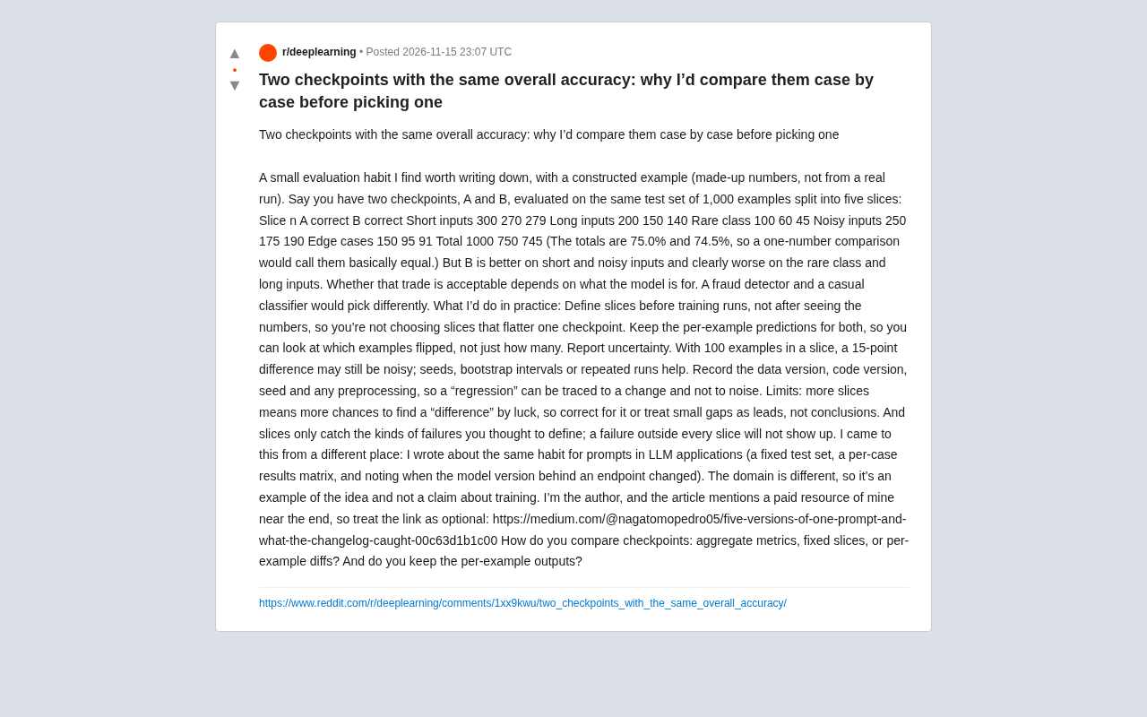
But the slice data tells a different story: B is better on short inputs and noisy inputs, and notably worse on rare categories and long inputs. This trade-off means which checkpoint to choose depends on what problem the model needs to solve—a fraud detector and a casual classifier would make completely different decisions.
Trade-offs Revealed by Slice Comparison
The slice data from the original post is as follows (all numbers fictional):
| Slice | Sample Count | A Correct | B Correct |
|---|---|---|---|
| Short inputs | 300 | 270 | 279 |
| Long inputs | 200 | 150 | 140 |
| Rare categories | 100 | 60 | 45 |
| Noisy inputs | 250 | 175 | 190 |
| Edge cases | 150 | 95 | 91 |
| Total | 1000 | 750 | 745 |
B gets 9 more correct on short inputs and 15 more on noisy inputs; but 15 fewer on rare categories and 10 fewer on long inputs. For scenarios that need coverage of rare categories (such as fraud detection), B's overall advantage is meaningless; for scenarios with short, noisy inputs, B may be the better choice.
The value of this example lies not in the numbers themselves, but in the evaluation mindset it demonstrates: overall metrics are a weighted average of slice performance, with weights determined by the test set distribution—and the test set distribution may not match the real business distribution.
Four Evaluation Habits in Practice
The original author offers practices he believes are worth maintaining. These suggestions target training checkpoint comparison, but the ideas can be transferred.
Define slices before training. If you divide slices after seeing the numbers, it's easy to pick a slicing that favors a particular checkpoint. Pre-defining slices locks in evaluation dimensions in advance, avoiding post-hoc selection bias.
Keep per-example prediction results. Don't just look at how many each slice got right—look at which specific samples flipped. Per-example comparison can answer qualitative questions like "where is B better than A, and where is it worse," while aggregate numbers can only answer "by how much."
Report uncertainty. The original post specifically mentions that with only 100 samples in a slice, a 15 percentage point difference could still be noise. Seed variation, bootstrap intervals, or repeated runs can all help determine whether a difference is stable.
Record data version, code version, seed, and preprocessing. This way, when a "performance regression" appears, you can trace it to a specific change rather than attributing it to random fluctuation.
Uncertainty quantification here refers to the statistical judgment of whether observed metric differences exceed the range of random fluctuation. In machine learning evaluation, the test set itself is just one sample drawn from the data distribution, so any metric carries sampling error. Common quantification methods include: bootstrap resampling (drawing multiple subsets from the test set with replacement, computing the empirical distribution of the metric to obtain confidence intervals), repeated training and evaluation with multiple random seeds (observing the variance of metrics under different initializations), and standard error estimation based on the binomial distribution (for accuracy, the standard error is approximately sqrt(p(1-p)/n)). When the metric difference between two models is smaller than the confidence interval width, you cannot assert that one model is truly better than the other. The original post's statement that "a 15 percentage point difference on 100 samples could be noise" is exactly an embodiment of this principle: at n=100, the standard error of accuracy is about 5%, and a 15 percentage point difference is only about 3 standard errors, which is not robust under multiple comparisons.
The Boundaries of the Slice Method
The author also candidly points out the limitations. The more slices you have, the greater the chance of finding a "significant difference" by luck, so multiple comparison correction is needed—or small gaps should be treated as clues rather than conclusions.
A more fundamental limitation: slices can only capture failure types you thought to define. If a failure mode isn't in any slice, it won't show up in the evaluation. This means slice design itself is an expression of domain knowledge, not a purely mechanical operation.
The author mentions he transferred this habit from another context: in LLM applications, creating fixed test sets for prompts, per-example result matrices, and recording changes in the model version behind an endpoint. He emphasizes that the domain is different, so this is just an illustrative example of the approach, not a claim about model training.
Multiple comparison correction is a method in statistics used to control the risk of "false positives." When performing multiple hypothesis tests simultaneously (for example, comparing two models across multiple slices), even if the significance level for each test is set at 0.05, the probability of at least one false positive across 20 independent tests is as high as about 64%. Common correction methods include Bonferroni correction (dividing the significance threshold by the number of tests) and the Benjamini-Hochberg procedure (controlling the false discovery rate, FDR). In slice evaluation, this means that if you define many slices and compare them one by one, you need to adjust the significance criteria—otherwise it's easy to mistake random fluctuation for a real difference. The original post's suggestion to "treat small gaps as clues rather than conclusions" is exactly a simplified expression of multiple comparison thinking in engineering practice.
What This Means for Evaluation Workflows
The original post ends with an open question: how do you compare checkpoints—aggregate metrics, fixed slices, or per-example differences? Do you keep per-example outputs?
There's no standard answer to this question, but the signal the post conveys is clear: when two checkpoints have similar overall metrics, the per-example and slice perspectives provide far richer decision-making evidence than a single scalar. For scenarios that require the model to be reliable on specific subpopulations, this fine-grained comparison isn't optional—it's a necessary step.
The author mentions at the end that his article contains links to paid resources, and notes that the links are optional.
One-line Summary
Checkpoints with similar overall accuracy may perform very differently at the slice level; decisions should combine per-example comparison with uncertainty reporting.
Paragraph Summary
The article uses a fictional example to illustrate: two models differ by only 0.5 percentage points in overall accuracy (75.0% vs 74.5%), but their performance trades off across five slices—Model B is better on short and noisy inputs, and notably worse on rare categories and long inputs. Therefore which checkpoint to choose depends on the application scenario. The author proposes four evaluation habits: define slices before training to avoid post-hoc selection bias, keep per-example prediction results to reveal flipped samples, report uncertainty to determine whether differences are stable, and record data and code versions for traceability. The article also points out the boundaries of the slice method: the more slices, the easier it is to find significant differences by luck, requiring multiple comparison correction; and slices can only capture failure types you thought of in advance, leaving coverage blind spots.
Related articles

ClawDOS: Bringing AI Coding Capabilities to DOS
ClawDOS is an AI coding agent project for DOS, exploring the possibility of bringing AI coding assistance into resource-constrained retro computing environments. This article analyzes its positioning, use cases, and community response.

Baseten Releases Bison-1 and Groundhog-1, Topping the Decision Model Leaderboard
Baseten releases open-weight decision models bison-1 and groundhog-1 built on Gemma 4; bison-1 scores 76 on the AA Decision Index v2.1 to top the leaderboard. Both support 128k context and image input—here we analyze their capability combination, benchmark significance, and selection advice for developers.

Cline CLI v3.0.75 Released: Yolo Mode Now Default for One-Shot Runs
Cline CLI v3.0.75: one-shot runs now default to yolo mode, --timeout and Ctrl+C can interrupt the first round, read_files is no longer truncated to 8k chars, plus reasoning parameter fixes and 94 new providers.