Scaling Laws for Pre-training and RL: Chess Experiments Reveal Post-Training Compute Allocation Principles

In the training pipeline of large models, how to allocate compute across the three stages—pre-training, SFT (Supervised Fine-Tuning), and RL (Reinforcement Learning)—has long been an open question without clear answers. In the pre-training era, we had the Chinchilla Law as guidance—roughly allocating 20 tokens per parameter for compute budgeting. The Chinchilla Law originated from DeepMind's 2022 research, with the core finding that under a fixed compute budget, model parameters and training data should scale proportionally. This overturned the GPT-3 era "bigger is better" mindset—where the industry favored training the largest possible models even with insufficient data. The Chinchilla Law demonstrated that a 70B parameter model trained on only 300B tokens might underperform a smaller model with sufficient training data. However, this law only covers the pre-training stage. When training enters the RL phase, how much compute to invest and what returns to expect has remained without clear guiding principles.

The paper recently discussed at the Hugging Face Journal Club attempts to answer precisely this question. It cleverly selects chess as the experimental platform, systematically studying how pre-training compute allocation affects downstream task performance in the post-training stage.

Building a Three-Stage Experimental Framework with Chess

The paper's experimental design is quite elegant, using chess as a "harness" to fully reproduce the pre-training, SFT, and RL stages.

Pre-training stage: Researchers collected large amounts of human chess game data. A game is essentially a sequence of moves (such as E2, E4, G5, etc.), and the model performs autoregressive training on these sequences—completely consistent with the pre-training logic of language models. Autoregressive training is the core training paradigm of current mainstream large language models, where the model learns to predict the next token in a sequence. The GPT series, LLaMA, Claude, and other models all adopt this approach. Chess games naturally fit this paradigm—each move can be encoded as a token, and an entire game becomes an ordered token sequence. The elegance of this analogy lies in the fact that chess sequences have strict causal structure (earlier moves determine later legal moves), perfectly matching the logic of context determining subsequent content in natural language, giving the experimental conclusions potential for transfer to language tasks.

SFT stage: This step features a novel design. Researchers use the pre-trained model to sample K trajectories from a given board position S0. Since these trajectories share some prefix moves, they naturally form a tree structure. The researchers then "linearize" this tree into Chain-of-Thought (CoT) data for model training. Chain-of-Thought is a technique that has models show intermediate reasoning steps before giving a final answer, proposed by Google researchers in 2022 and now a standard method for improving model reasoning capabilities.

A notable detail: this CoT construction method differs from approaches used in LLM tasks like DeepSeek^Ad-R1. DeepSeek-R1's chain-of-thought resembles free-form internal monologue, while the CoT here is structured—the model explicitly explores multiple candidate move sequences and then selects the optimal one. This design teaches the model a "explore first, decide later" pattern, similar to Monte Carlo Tree Search (MCTS) in spirit, but embedded in the Transformer's generation process in a serialized manner.

RL stage: This step also features unique reward design. The model starts from a given board state, performs reasoning, and outputs the next move. The reward mechanism works as follows: if the model doesn't play the optimal move for the current state, it scores zero; if it plays the optimal move, it advances to the next state. Only when every move along the entire trajectory is optimal does the model receive a full score of 1. The "optimal move" is determined in real-time by chess engines like Stockfish. Stockfish is one of the world's strongest open-source chess engines, with an Elo rating exceeding 3500 (far surpassing the human world champion's approximately 2850), based on alpha-beta search algorithms and NNUE (Efficiently Updatable Neural Network Evaluation), capable of determining the optimal move for any position in extremely short time.

This process-level supervision differs fundamentally from traditional RL that only scores final trajectories. It provides reward signals step-by-step, move-by-move, avoiding the sparse reward problem when an entire game is treated as a single trajectory. This aligns with OpenAI's approach of using Process Reward Models (PRM) in mathematical reasoning—evaluating each reasoning step individually rather than only checking whether the final answer is correct, thereby dramatically improving learning efficiency.

Core Finding: More Pre-training Compute Means Stronger Downstream Performance

The paper's most important conclusions center on the relationship between downstream task performance and compute allocation.

First, the more compute allocated to pre-training, the higher the downstream pass@1 reward. Lower pre-training loss means stronger model generalization, yielding greater returns from subsequent RL. This is intuitively reasonable—a better base model means a higher performance ceiling.

Second, and most intriguing: RL can significantly improve pass@1 but has almost no impact on pass@k, regardless of pre-training scale. Understanding these two metrics is essential: pass@1 measures the probability of the model generating the correct answer on a single attempt, reflecting reliability and certainty; pass@k measures the probability of getting at least one correct answer across k independent samples, reflecting the model's capability ceiling and solution space coverage. The gap between them reveals the difference between a model's intrinsic capability and output consistency—a model with high pass@16 but low pass@1 "knows" the correct answer but cannot reliably output it.

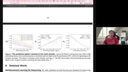
From the charts, the experiments distinguish several key elements: RL trajectories (solid lines), Step 0 (pre-training + SFT, circle markers), the Pareto frontier, and RL compute fraction. The Pareto frontier is a classic concept in multi-objective optimization, referring to the set of optimal solutions where no other solution can improve one objective without degrading another. When fixing total compute budget: if you simply keep expanding pre-training compute, pass@k improves linearly; but if you take one point and allocate a portion of compute (say 30%) to RL, you get dramatic improvements—for example, jumping from 10 to 30 on pass@k.

In other words, RL delivers vertical performance gains. On the pass@16 metric, the Step 0 circles are already nearly on the Pareto frontier, with limited RL benefit; but on pass@1, models of all scales benefit significantly from RL. RL's improvement of pass@1 without affecting pass@k is essentially "compressing" the model's output distribution, concentrating it more around the correct answer—so-called distribution sharpening.

This is profoundly significant. The pass@1 improvement means enhanced model reliability—it not only occasionally produces correct answers but can more consistently get things right on the first try. This may partially explain why some models achieve dramatic performance leaps merely through adjusting post-training strategies.

Smaller Models Trained Longer Beat Larger Models

Analysis in the paper's appendix reveals a phenomenon that contradicts the Chinchilla Law. Researchers plotted pre-training loss against parameter count, forming a "valley" shape. They found: for a fixed compute budget, training a smaller model for longer often outperforms training a larger model.

Specifically, within the compute ranges they explored, the 1-billion parameter model's pass@1 performance was almost always inferior to smaller models. The Chinchilla-optimal ratio (dashed line in the figure) was not the best choice. Of course, discussants cautiously noted that this conclusion may relate to the specifics of chess—after all, chess has a vocabulary of only about 81 tokens, while natural language vocabularies are hundreds to thousands of times larger (typically 32,000 to 100,000+), with potentially very different distribution dynamics. In a small-vocabulary environment, the model doesn't need massive parameters to "memorize" token embeddings, so parameter utilization efficiency is higher, and the marginal returns from longer training may be greater.

Is RL "Sharpening" Existing Capabilities or Creating New Ones?

A profound question in the discussion: what exactly does RL bring to the model?

The paper's conclusion is "mixed." On one hand, for problems the base model can already solve, RL amplifies these capabilities, making model outputs more consistent (explaining the pass@1 improvement with unchanged pass@k); on the other hand, on difficult positions, RL can occasionally enable the model to find good moves that the base model could almost never discover.

The discussants' consensus: if the base model has a 0% success rate on pass@16, RL is almost incapable of creating new capability from nothing; but as long as there's a non-zero success probability, RL can enhance and amplify it. The paper's analysis by problem difficulty confirms this—on easy problems, RL amplifies good solutions; on hard problems, it sometimes achieves "tail discovery" of good moves outside the distribution, but sometimes merely reinforces the model's known, potentially incorrect answers.

Practical Implications and Limitations

The paper's greatest value lies in its clean, controlled experimental design—fixing data and only varying compute to derive clear compute-performance relationships. But discussants also frankly noted its limitations for practical work.

For most practitioners, the real scenario involves taking an open-source pre-trained model (whose pre-training recipe is typically unknown) and performing RL or mid-training on top of it. Mid-training is a stage in the large model training pipeline that has gained increasing attention in recent years, positioned between general pre-training and task-specific fine-tuning, typically referring to continued pre-training with domain-specific data after pre-training is complete but before SFT/RLHF. For example, Meta's Code Llama was obtained by mid-training LLaMA 2 with large amounts of code data. The core value of mid-training lies in efficiently injecting domain knowledge—compared to training from scratch, it requires one to two orders of magnitude less compute but can significantly improve model performance in specific domains.

Thus the key question becomes: do these scaling laws apply to mid-training? If we cannot redo pre-training, can we derive similar curves based on mid-training loss?

The paper's experiments on math tasks (Figure 6) address precisely this question. Researchers trained a 1-billion parameter model with 200 billion tokens of Numeratron math and Dolma mixed corpus, demonstrating the relationship between mid-training loss and RL performance. This is considered the most practically relevant result—because it establishes a measurable connection between mid-training investment and downstream returns.

Discussants further raised a deep unresolved question: starting from random initialization (or random-level task performance), can RL "learn from zero"? Taking biology tasks as an example, most open-source models perform near random (50%) while frontier models get them right—indicating that frontier models learned certain critical knowledge. So should compute be invested in mid-training to inject domain knowledge, or directly in RL to amplify weak signals already present in the base model?

The consensus leans toward: RL is not good at creating capabilities from scratch. Although AlphaZero proved that RL from random initialization is viable in specific environments, its success has special prerequisites: game rules are completely known, the state space is large but bounded, reward signals are clear (win/loss), and the environment can be perfectly simulated allowing unlimited sampling. These conditions are almost never met in natural language tasks—language "rules" are implicit, the state space is nearly infinite, correctness judgment often requires external knowledge, and one cannot generate unlimited training data at zero cost as in board games. Therefore, while AlphaZero proved the theoretical feasibility of RL learning from scratch, transferring this paradigm to language models faces fundamental sample efficiency challenges. RL is more like a "sharpening" blade for capabilities, not a "sculptor" creating from nothing.

Conclusion

Although this paper is based on the constrained environment of chess, it provides a rare, clean quantitative framework for understanding the compute trade-offs between pre-training, SFT, and RL. It establishes several important principles: pre-training compute determines the downstream ceiling, RL primarily improves reliability (pass@1) rather than exploration breadth (pass@k), and smaller models may be preferable under fixed compute budgets.

However, as discussants repeatedly emphasized, whether these conclusions generalize to large-vocabulary natural language tasks and whether they can guide mid-training compute allocation still requires further research. For teams truly training models from scratch, this serves as a valuable reference recipe; for the majority of practitioners doing post-training on open-source models, the most practical guidance may still come from work directly studying RL trade-offs on fixed base models.