The Mean Reversion Trap: Why Churn Models Misclassify Growing Physicians

The Problem: Why Growing Physicians Get Flagged as Churn Risks

In the field of prescription and physician data analytics, building a Churn Risk Model is a common yet highly challenging task. Churn risk models are core predictive tools in customer lifecycle management, widely used across telecom, SaaS subscriptions, financial services, and the pharmaceutical industry. In Pharma Commercial Analytics, sales teams need to identify which physicians (Key Opinion Leaders or high-prescribing Healthcare Professionals) might reduce or even stop prescribing a particular drug. The model's output typically drives sales rep visit prioritization directly — if a high-value physician is predicted as a churn risk, the sales team will increase visit frequency, provide more academic support, or arrange Medical Science Liaison interventions. As a result, model mispredictions don't just waste resources — they can cause truly at-risk physicians to be overlooked.

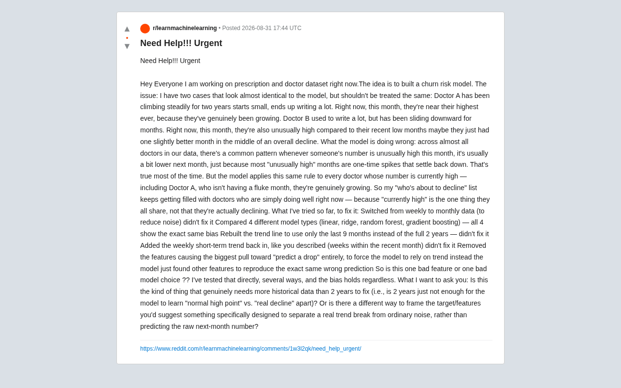
Recently, a data science practitioner shared a classic dilemma on Reddit: their model couldn't distinguish between two types of physicians who look similar on the surface but are fundamentally different.

Specifically:

• Physician A: Prescription volume has been steadily climbing over the past two years, growing from low to high. This month's value is near the historical peak — a result of genuine growth.
• Physician B: Once had high prescription volume, but it has been declining over recent months. This month's value happens to be high, but it's just a temporary bounce within an overall downward trend.

To the model, the feature "both physicians are currently at a high level this month" looks nearly identical, so they're treated equally — but from a business perspective, A is a healthy, growing customer, while B is the one who's actually a churn risk.

The Root Mechanism: Mean Reversion Makes the Model Treat Everyone the Same

The original author keenly identified the core mechanism at play:

"Across nearly every physician's data, there's a common pattern — when someone has an abnormally high number this month, it usually dips slightly the next month, because most 'abnormally high' months are one-time spikes that revert to normal afterward."

This is the classic Mean Reversion phenomenon in statistics. Mean reversion was first described by Francis Galton in the 19th century while studying the relationship between parents' and children's heights, and it later became a foundational concept in statistics and finance. Its core meaning is: if a variable shows an extreme value in one observation, it tends to return closer to its long-term average in the next observation. This isn't some mysterious force "pulling" the value back — it's because extreme observations typically contain a random fluctuation component. After a lucky month, the luck factor fades, and the value naturally drops. In medical data, physicians' prescribing behavior is similarly influenced by random factors like patient visit volume fluctuations, seasonality, and sample distribution cycles, so it naturally exhibits mean reversion characteristics.

During training, the model learns a universal rule: current value abnormally high → high probability of decline next month. This rule holds true in most cases, so the model indiscriminately applies it to all physicians currently at high levels — including Physician A, whose high value isn't a random fluctuation but genuine growth.

The end result: the "about to churn" prediction list gets filled with top-performing physicians, because "currently at a high level" is their only shared trait — not because they're actually declining.

Why Switching Models and Features Didn't Help

The author had already done extensive troubleshooting:

1. Switched from weekly to monthly data (to reduce noise) — no effect
2. Compared four models (Linear Regression, Ridge Regression, Random Forest, Gradient Boosting) — all four exhibited the exact same bias
3. Shortened the trend window from two years to the most recent 9 months — no effect
4. Re-added weekly short-term trends — no effect
5. Directly removed the strongest feature causing "predicted decline" — the model simply used other features to reproduce the same erroneous prediction

It's worth elaborating on the four models compared: Linear Regression, Ridge Regression, Random Forest, and Gradient Boosting. These span from the simplest linear parametric models to the most powerful ensemble learning methods. Linear Regression and Ridge Regression are parametric models that minimize the sum of squared residuals to fit linear relationships, with Ridge Regression adding L2 regularization to prevent overfitting. Random Forest reduces variance through Bagging ensembles of multiple decision trees, while Gradient Boosting (e.g., XGBoost, LightGBM) sequentially trains weak learners to progressively reduce bias. These four algorithms have fundamentally different inductive biases: linear models assume a linear relationship between features and target, while tree-based models can capture arbitrary nonlinear interactions. When such different algorithms all converge on the same error pattern, it's a strong signal in machine learning diagnostics — indicating that the problem lies not in model capacity or regularization strategy, but in a systematic flaw in the training data's label definition or feature space.

This series of experiments actually provided a clear answer: this is neither a bad feature problem nor a model selection problem. When four fundamentally different algorithms and multiple feature combinations all converge on the same bias, the problem lies at the Problem Framing level, not in implementation details.

The Fundamental Cause: The Prediction Target Is Defined Wrong

The author's current modeling approach is to predict the raw next-month prescription count. This target itself has the mean reversion trap baked in.

When you train a model to predict "next month's absolute value," the model naturally learns: high-value samples tend to regress. This is a real statistical pattern in the data, and no model swap can avoid it. In other words, the model isn't wrong — we asked the wrong question.

Problem Framing is the most underestimated yet most critical step in the machine learning project lifecycle. Google's ML engineering best practices guide lists it as the very first step of a project, even before data collection. It answers the fundamental question: "What exactly are we asking the model to predict?" A classic example: in recommendation systems, predicting "whether a user will click" versus predicting "whether a user will be satisfied" are two completely different objectives — the former leads to clickbait content being heavily recommended. Similarly, in this case, "predicting next month's absolute prescription count" and "predicting whether a physician is churning" may seem related, but they guide the model in entirely different directions. A wrong problem definition causes all subsequent feature engineering, model tuning, and hyperparameter search to be meticulously optimized in the wrong direction — creating a kind of "precise wrongness."

What truly needs to be distinguished isn't "will next month's number be lower," but rather "is this physician on a healthy growth trajectory or a structural decline trajectory?" The difference between the two lies not in whether the current value is high or low, but in the direction, acceleration, and consistency of the trend.

Solution Approach: Redesigning the Target and Feature Engineering

Rather than obsessing over data volume, the right move is to redesign the modeling paradigm from the ground up.

Redefine the Prediction Target

Don't predict raw values. Instead, predict trend breaks or deviations from each physician's own baseline. Specific methods include:

• Use each physician's own historical trajectory as the baseline, predicting whether future values will significantly fall below their personal trend line, rather than comparing absolute levels
• Reframe the target as a classification problem: "Will this physician experience a structural decline in the next N months?" — labeled using explicit business rules
• Use detrended residuals as the analysis target, stripping away each physician's individual baseline

Detrending is a standard preprocessing step in time series analysis, designed to strip the long-term trend component from the raw series and retain only the fluctuations around the trend (i.e., residuals). Common detrending methods include: differencing (first-order differencing converts absolute values to period-over-period changes), linear or polynomial regression detrending (fitting a trend line and taking residuals), and more flexible approaches like the Hodrick-Prescott filter or STL decomposition (decomposing the series into trend, seasonal, and residual components). In this case, performing detrending individually for each physician's prescription series means the model no longer sees "Physician A prescribed 200 scripts this month" but rather "Physician A is 5 scripts above their own trend line this month." This way, a physician in an upward channel may show normal residuals even at a high current value, while a physician in a downward channel will show an abnormally high residual even during a single high month — the two look completely different in residual space.

Build Features That Distinguish "Growth" from "Decline"

The key is to let the model see the shape of the trend, not just the current level:

• Trend slope and its sign: The regression slope over the past N months — positive or negative sign directly distinguishes Physician A from Physician B
• Trend consistency: The number of consecutive months of increase or decrease, or the trend's R² (goodness of fit)
• Current value's position relative to the individual's long-term trend line: A's current value aligns with their upward trend line; B's current value clearly deviates from their downward trend line
• Acceleration features: The difference between the recent slope and the earlier slope, used to capture trend inflection points

Fitting a simple linear regression line to each physician's historical prescription series yields two key pieces of information: slope and R². The sign of the slope directly encodes the direction of growth or decline — a positive slope means prescription volume is increasing over time, a negative slope means it's decreasing. The absolute value of the slope reflects the rate of change. R² (coefficient of determination) measures how well the trend line explains the actual data, ranging from 0 to 1. An R² near 1 indicates the physician's prescribing behavior is very consistently following the trend direction with minimal fluctuation; an R² near 0 indicates the trend is unclear and the data is primarily driven by random fluctuation. Using both in combination: positive slope + high R² = stable growth (Physician A's typical profile); negative slope + low R² = downward trend interspersed with bounces (Physician B's typical profile). This feature design compresses time series shape information into scalar features the model can directly use.

Physician A has a positive slope and high trend consistency; Physician B has a negative slope, and the current value is just a bounce within a declining channel. Once these features enter the model, the two no longer "look the same."

Normalize at the Individual Physician Level

Since each physician's baseline level varies enormously, it's recommended to standardize features at the individual level (e.g., Z-scores relative to each physician's own historical mean and standard deviation).

The Z-score formula is Z = (X - μ) / σ, where μ is the mean and σ is the standard deviation. When this calculation is performed at the individual physician level — using that physician's own historical mean and standard deviation — it achieves a "personalized baseline" effect. For example, a community general practitioner might average 20 prescriptions per month, while a department chief at a large hospital might average 200. If measured by a single global standard, the 200-prescription physician will always appear "high" and the 20-prescription physician will always appear "low," and the model will primarily learn scale differences between physicians rather than individual behavioral changes. With individual Z-scores, the model focuses on "how much this physician deviates from their own norm," placing physicians of different scales on the same comparable axis. This approach is also common in recommendation systems — for example, Netflix subtracts each user's average rating before modeling preference differences.

This way, the model judges not "is the absolute value high" but "is this abnormal relative to their own historical performance."

Data Volume Isn't the Bottleneck — Problem Definition Is

The author's final question was: is two years of data simply not enough for the model to learn to distinguish "normal peaks" from "genuine decline"?

The answer: data volume isn't the main bottleneck — problem definition is. More historical data certainly helps estimate each physician's trend and fluctuation range more robustly, but if the target remains "predict next month's raw value," more data will only reinforce the mean reversion pattern.

The fundamental fix is to correct the modeling paradigm first — shifting from predicting raw values to identifying trend breaks, and introducing directional features. On that foundation, longer historical data becomes the icing on the cake.

Conclusion

This case is a highly representative lesson in data science: when every model and every feature adjustment points to the same error, the answer usually lies above the modeling layer — in how you defined the problem itself. Mean reversion is an objective statistical pattern in the data; trying to "suppress" it with modeling tricks is futile. The correct approach is to redesign the prediction target and feature system so the model answers the business question you actually care about.