Transformer Attention Mechanism Deep Dive: From Tokens to Self-Attention, Step by Step

Understanding the long-context processing capabilities of large language models and AI agents requires a solid grasp of Transformer's underlying architecture. Many techniques for optimizing agent long-context handling trace their roots back to the Transformer itself — and especially its core attention mechanism. This article systematically walks through the complete pipeline from text input to self-attention computation, helping readers understand the data flow and dimension changes at every step.

From Text to Vectors: Tokenizer and Embedding

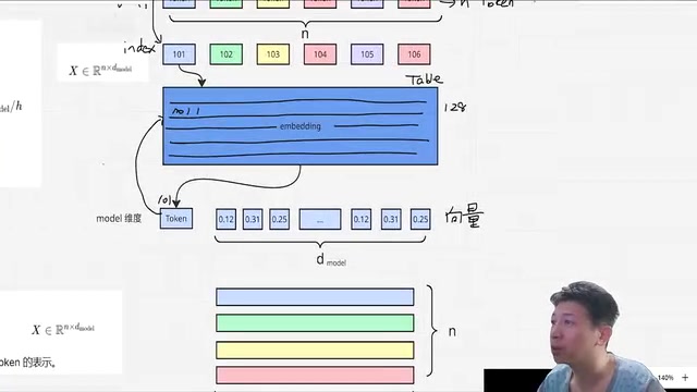
When we feed a sentence to a Transformer — say, "Give me a brief introduction to the Transformer attention mechanism" — the model first runs it through a Tokenizer. The way the model splits text differs subtly from how humans read: spaces are treated as part of token units, whereas human readers tend to ignore them automatically. The result of tokenization is a sequence of N tokens — the smallest semantic units a language model works with.

At this point, tokens are still character-level symbols (Chinese characters or English letters). The next critical step is encoding: during tokenization, each token is already mapped to an ID (for example, the word "简单" might be assigned ID 101 — this is just illustrative). Given an ID, the model looks up a pre-trained dictionary table called an Embedding Table, retrieving a vector at the corresponding position.

This table is itself learned during training. After the lookup, characters become vectors, and the dimensionality of each vector is determined by the table — typically called d_model, which might be 128, 256, or 1024. Once all N characters are each converted to a d_model-dimensional vector, the entire input sentence becomes an N × d_model matrix. With 6 characters and 128 dimensions, for instance, the input matrix is 6 × 128. This step is the starting point for all subsequent matrix operations — keep a close eye on how dimensions shift.

---

The specific tokenization strategy has a profound impact on model performance. Leading large language models overwhelmingly use subword algorithms like BPE (Byte Pair Encoding) or SentencePiece, rather than naively splitting by character or word. BPE starts from individual characters and repeatedly merges the most frequent adjacent character pairs in the corpus, ultimately building a vocabulary of tens of thousands to hundreds of thousands of entries. The benefit is a balance between vocabulary size and expressive power: high-frequency words appear as complete tokens, while rare or unseen words are broken into smaller subword fragments — drastically reducing the "out-of-vocabulary" problem. Vocabulary sizes vary considerably across models: GPT-4 uses roughly 100,000 entries, while the LLaMA series uses around 32,000. This directly affects how many tokens a given passage is split into, which in turn affects how many characters can actually fit inside a context window. Understanding tokenization helps explain why the same number of characters in Chinese and English can consume very different numbers of tokens — Chinese characters typically map to 1–2 tokens each, while English words may be split into multiple subword fragments.

The Intuition Behind Self-Attention: Q, K, and V

With the input matrix X (N × d_model, abbreviated as dm), the model moves into attention computation. Three learnable weight matrices are introduced to transform each token's vector into a Query, a Key, and a Value respectively. These weight matrices compress the dm-dimensional vectors down to dk dimensions, so X multiplied by each weight matrix goes from N × dm to N × dk.

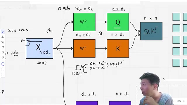
Why distinguish between Q, K, and V? The core reason is to compute relationships between words. A word in isolation carries incomplete meaning — it needs to absorb information from surrounding words to enrich its representation. The mechanism works like this: when word A wants to gather information, it takes its Query and multiplies it against word B's Key, producing a weight (a relevance score) — say, A and B have a relevance of 0.1, while a more distant word C scores 0.05. These weights are then applied to the other words' Values (which are abstract representations of their meaning), and A "absorbs" information from other words in proportion to those weights, blending it into its own representation.

At a high level, all N words must compute pairwise relevance with each other, so Q multiplied by the transpose of K produces an N × N matrix where each element represents the relationship strength between two words.

---

The names Q, K, and V are borrowed from the field of information retrieval. The entire attention mechanism can be thought of as a soft database query: the Query is your search request, the Key is the index label on each database record, and the Value is the actual content of that record. You compute similarity between the Query and every Key to get a match score for each record, then take a weighted sum of all Values according to those scores to produce the query result. Unlike hard retrieval (which returns only the single best match), attention is "soft" — all Values participate in the aggregation, just with varying weights — making gradients flow through and enabling end-to-end training. This ability for every word to attend to all other words simultaneously is what gives Transformer its global perspective and allows it to capture long-range dependencies. This is also its core advantage over RNNs: an RNN must pass information step by step, and distant information can fade during transmission. Self-attention treats interactions between any two positions in the sequence as equivalent, with no distance-based decay.

The Mask Mechanism: Why the Model Can't See the Future

After computing the N × N weight matrix, a Mask needs to be applied. The reason is that language generation is sequential — words are produced one at a time: first "简单", then "介绍", then "Transformer". When the model is processing the word "介绍", it should only be able to see "简单" and itself — not any of the words that haven't been generated yet.

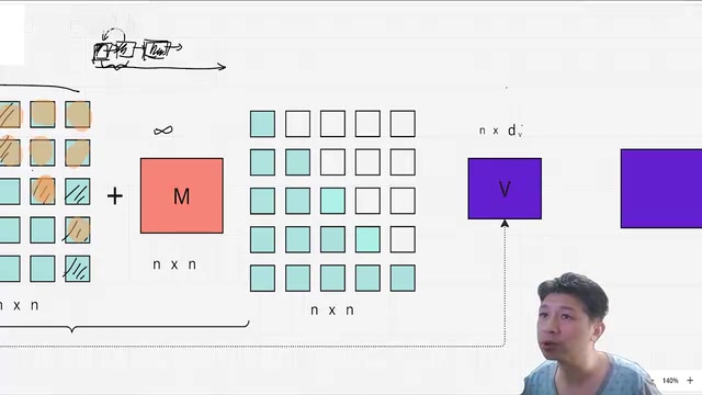
The Mask is an N × N matrix. Positions that need to be blocked (i.e., all positions after the current word) are set to negative infinity. When this Mask matrix is added to the relevance matrix S, the negative-infinity positions approach zero after Softmax — effectively being "erased". This creates a natural causal generation effect: when position j > i, the value is negative infinity; when j ≤ i, the original value is kept. This is precisely why a Mask must be introduced in Decoder scenarios.

Breaking Down the Formula: Tracking Dimensions Step by Step

Putting the intuition into formulas, tracking dimensions carefully is essential. The input X has shape N × dm. Multiplying by two weight matrices gives Q and K, both with shape N × dk.

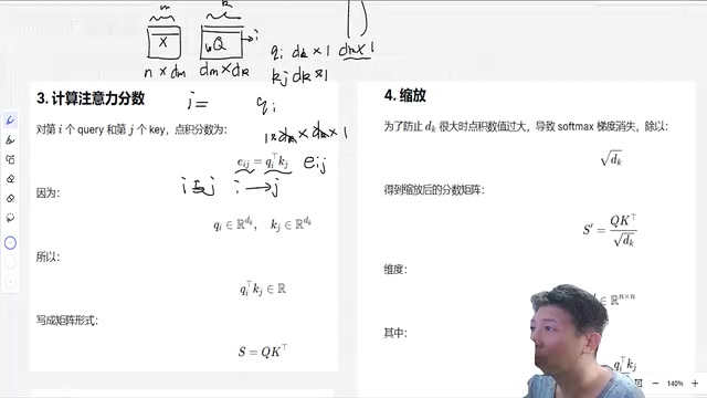
To compute relevance, Q (N × dk) is multiplied by the transpose of K (dk × N). The dk dimension cancels out, yielding the score matrix S with shape N × N. There's also a scaling factor: dividing by the square root of dk. When dk is large, dot products can become very large, causing Softmax gradients to vanish — so scaling by the dimension size is necessary, giving S'.

Next, the Mask matrix (also N × N) is added, setting positions to be blocked to negative infinity, yielding S''. Softmax is applied to S'', turning each row into a probability distribution that sums to 1 — this is the actual attention weight matrix A (N × N). It's worth noting that Softmax carries significant computational complexity; many long-context optimization approaches focus precisely on how to simplify or replace this step.

Finally, the weight matrix A (N × N) is multiplied by V (N × dv) to produce the output O (N × dv). An output weight matrix Wo then projects the dimensions back to N × dm. A residual connection with the original input X ensures the output dimension remains N × dm, ready to serve as input to the next layer. Stacking these layers allows information to be progressively enriched, forming the complete Transformer architecture.

---

Residual connections and layer normalization are key engineering choices that allow Transformer to stably stack dozens or even hundreds of layers, and deserve special mention. Residual connections originate from ResNet; their formula is output = F(x) + x — the current layer's transformed output is added directly to the input, providing a "highway" for gradients and effectively mitigating the vanishing gradient problem in deep networks. Layer normalization independently normalizes each sample across its feature dimension to zero mean and unit variance, stabilizing the numerical distribution of each layer's input and making training less sensitive to learning rate choice. In the original Transformer (Post-LN), normalization is applied after the residual addition; many modern large models (such as LLaMA) switch to Pre-LN or RMSNorm, placing normalization before the transformation for even greater training stability. Together, these two mechanisms ensure that attention outputs, after the residual connection, remain at N × d_model in shape while staying numerically well-behaved, allowing signals to flow cleanly into the next layer.

Summary

The complete pipeline can be summarized as: text → tokens → IDs → embedding vectors → input matrix → Q/K/V projections → relevance computation → scaling → Mask → Softmax → weighted aggregation of V → output projection → residual connection. Tracking the dimension at each step is the key to understanding the attention mechanism. With this foundation in place, you'll be well equipped to understand the design motivations behind downstream engineering techniques such as KV Cache, long-context optimization, and Softmax approximations.

---

KV Cache is one of the most important engineering optimizations when applying the attention mechanism to autoregressive inference, and its principles build directly on the complete pipeline described above. During token-by-token generation, each new token theoretically requires recomputing K and V for the entire sequence generated so far. But since the K and V values of past tokens don't change during generation, they can be cached. A new token only needs to compute its own Q, dot it against all cached historical K values, and then take a weighted sum over all cached V values — avoiding redundant computation entirely. The cost of KV Cache is that memory usage grows linearly with sequence length: cache size is 2 × N × d_model × num_layers (the factor of 2 accounts for both K and V). This is the primary source of memory pressure in long-context inference, and the core motivation behind optimizations like KV Cache quantization, Multi-Query Attention (MQA), and Grouped-Query Attention (GQA).