Understanding KV Cache: The Space-Time Tradeoff Behind LLM Inference Optimization

What Is KV Cache

KV Cache (Key-Value Cache) is a core optimization technique used during the inference phase of large language models. At its heart, it's a space-for-time tradeoff. In autoregressive generation, the model predicts one token at a time, and each new token requires an Attention computation. Without any caching, every generation step would recompute the Key and Value vectors for every previously generated token — a massive waste of compute that grows worse with longer sequences.

The solution is straightforward: cache the K and V vectors of already-processed tokens in GPU memory. When generating each new token, the model only needs to compute Q, K, and V for that single new token, then concatenate them with the cached history to complete the attention calculation — eliminating all redundant recomputation.

The Computation Flow Without Caching

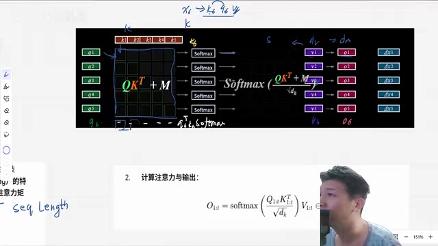
To appreciate the value of KV Cache, it helps to understand what happens without it. Recall the basic attention mechanism: the model has three weight matrices — Q, W_Q, W_K, and W_V — and input tokens are projected through these weights to produce Query, Key, and Value vectors. During attention, the Query performs dot products with all Keys to produce relevance scores, which are softmax-normalized and used to compute a weighted sum of the Value vectors. The result is a new representation for each token, followed by a linear projection to produce the final output.

The problem lies in autoregressive token-by-token generation. Suppose 5 tokens have already been generated and the model is now producing the 6th token X6. The model computes Q6, K6, and V6, then takes dot products between Q6 and K1 through K6 to get attention weights. But here's the key issue — the K and V vectors for X1 through X5 were already computed in previous steps and haven't changed at all. Recomputing all existing tokens' attention from scratch every time a new token is added is exactly where the waste occurs.

Autoregressive generation is the core decoding paradigm of today's mainstream large language models (such as the GPT series): the model generates one token at a time, appends it to the input sequence, then uses the extended sequence to predict the next token — repeating until an end token is reached. This serial, incrementally expanding mechanism inherently introduces heavy redundant computation, as the number of historical tokens participating in attention grows linearly with sequence length. Non-autoregressive models attempt to generate all tokens in parallel, but typically fall short in output quality. Because autoregressive generation is unavoidable, KV Cache has become the standard tool for accelerating Transformer inference.

How Caching Is Implemented

Since the projection results for historical tokens are reusable, the idea is simply to save them. The full sequence computation can be split into two parts: the historical portion from step 1 through T-1, and the newly added T-th token.

For the Query matrix, its dimensions are N×D_k, where N is the sequence length and D_k is the vector dimension of each representation. The input X (shape T×D_m) is multiplied by the weight matrix W_Q (shape D_m×D_k) to produce a Q matrix of shape T×D_k. A critical property here is that the projection is independently decomposable per token — a single token X_i (shape 1×D_m) multiplied by W_Q yields its own 1×D_k output. This per-token independence is precisely what makes caching possible.

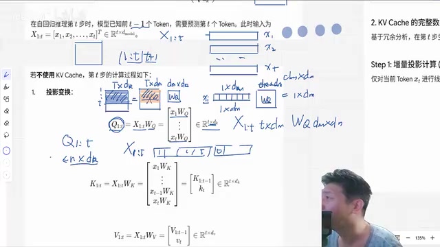
The same applies to Key and Value — each newly computed token's K and V are saved into the cache. This means the historical K and V vectors already reside in GPU memory and don't need to be recomputed.

Computing a New Token with KV Cache

When a new token X_T arrives, the process is dramatically simplified:

• Compute Q_T for the new token, producing a 1×D_k vector (effectively adding one new row to the Q matrix);
• Compute K_T and V_T for the new token, one row each;
• Concatenate the new K_T and V_T with the cached historical K and V;
• Take dot products between the newly computed Q_T and all concatenated K vectors to produce a 1×T weight vector representing the current token's relevance to every historical position;
• Apply softmax normalization to this weight vector (softmax is only computed for this single new row — the historical portion requires no recomputation);
• Multiply the normalized weights by the concatenated V matrix (shape T×D_v) to produce a 1×D_v output — the attention result for the T-th token.

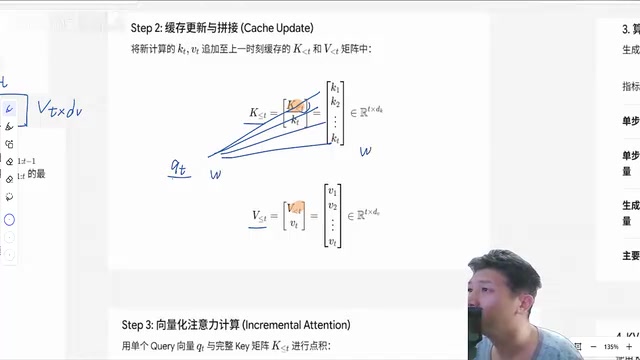
For comparison: without caching, each step requires computing a full N×D_k Q matrix projection; with KV Cache, only a 1×D_k computation is needed per step. The gap in compute grows dramatically as sequence length increases.

Time Complexity Comparison

Looking at time complexity makes the benefit even clearer. Let the input token length be N and the hidden dimension be D (assuming D_m equals D_k for simplicity).

Without caching: The projection computation (X multiplied by W_Q to produce a T×D Q matrix) has complexity roughly T·D²; the self-attention computation of Q (T×D) multiplied by the transpose of K (D×T) to get T×T has complexity roughly T²·D. Summed across all N generation steps, the total scales approximately as N²·D² + N³·D.

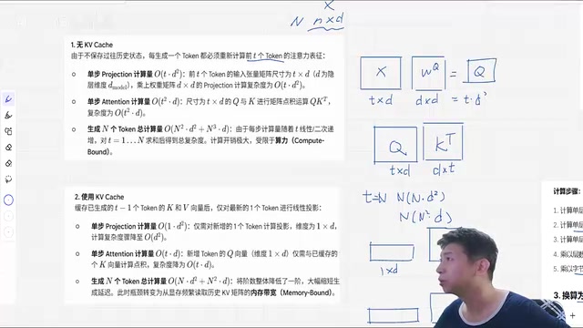
With KV Cache: Each step only computes a single new token rather than the full sequence. The projection reduces from T to a constant 1, and the attention computation only involves the new token interacting with the cached history. The overall complexity drops significantly to a much lower order. The longer the sequence and the more tokens generated, the more dramatic the speedup from KV Cache becomes.

Estimating Memory Overhead

The cost of saving time is GPU memory consumption. KV Cache memory overhead can be estimated with the following formula:

Memory_cache ≈ 2 × num_layers(L) × num_heads × head_dim × sequence_length × bytes_per_element

The factor of 2 comes from needing to cache both K and V. As a concrete example: L=32 layers, 32 attention heads, head dimension 128 (hidden dim 4096 ÷ 32 heads = 128), and sequence length S. Plugging in these values and multiplying by the byte size of the numerical precision gives the GPU memory required to store the K and V cache.

Memory overhead scales linearly with number of layers, number of heads, head dimension, and sequence length. This explains why long-context inference becomes a memory bottleneck — the longer the sequence, the more linearly KV Cache memory grows, making it a critical tradeoff in large model deployment.

Using LLaMA-2 7B as a concrete reference: L=32 layers, 32 attention heads, head dimension 128. With FP16 (2 bytes) precision at sequence length 2048, KV Cache occupies approximately 2 × 32 × 32 × 128 × 2048 × 2 ≈ 1.07 GB of GPU memory. When the context extends to 32K tokens, this number balloons to roughly 16 GB — close to the total memory of a single consumer-grade GPU. This is precisely why the industry has developed memory-compression techniques targeting KV Cache, such as PagedAttention (vLLM), Multi-Query Attention (MQA), and Grouped-Query Attention (GQA). MQA has all attention heads share a single set of K and V projections; GQA groups multiple heads to share K and V projections — both achieve a better balance between memory usage and model expressiveness.

Summary

KV Cache is an essential optimization that no serious LLM inference setup can ignore. By caching the Key and Value vectors of historical tokens, it reduces each generation step's redundant computation to only what's needed for the new token — trading GPU memory for generation speed. Understanding KV Cache not only helps in grasping the performance bottlenecks of Transformer inference, but also lays the groundwork for exploring advanced optimizations like PagedAttention and quantized caching. The memory pressure it introduces is, in turn, the central battleground for engineering optimization in long-context inference scenarios.