vLLM P/D Disaggregation: The Calculation Rule Where KV Transfer Cost Determines Benefit

Why P/D Disaggregation Is an Architectural Choice Worth Calculating Carefully

Splitting prefill and decode onto separate engine instances is one of the deployment patterns vLLM has pushed heavily in recent years. But the official vLLM documentation puts it quite bluntly: P/D disaggregation allows independent tuning of time-to-first-token (TTFT) and inter-token latency (ITL), and enables more reliable control of ITL tail jitter, but "disaggregated prefill does not improve throughput."

This means P/D disaggregation is fundamentally a latency engineering tool, not a throughput optimization. The price you pay is that every request's KV cache must be transported over the network from the prefill instance to the decode instance. Whether this trade pays off depends on your network, your model, and your request distribution.

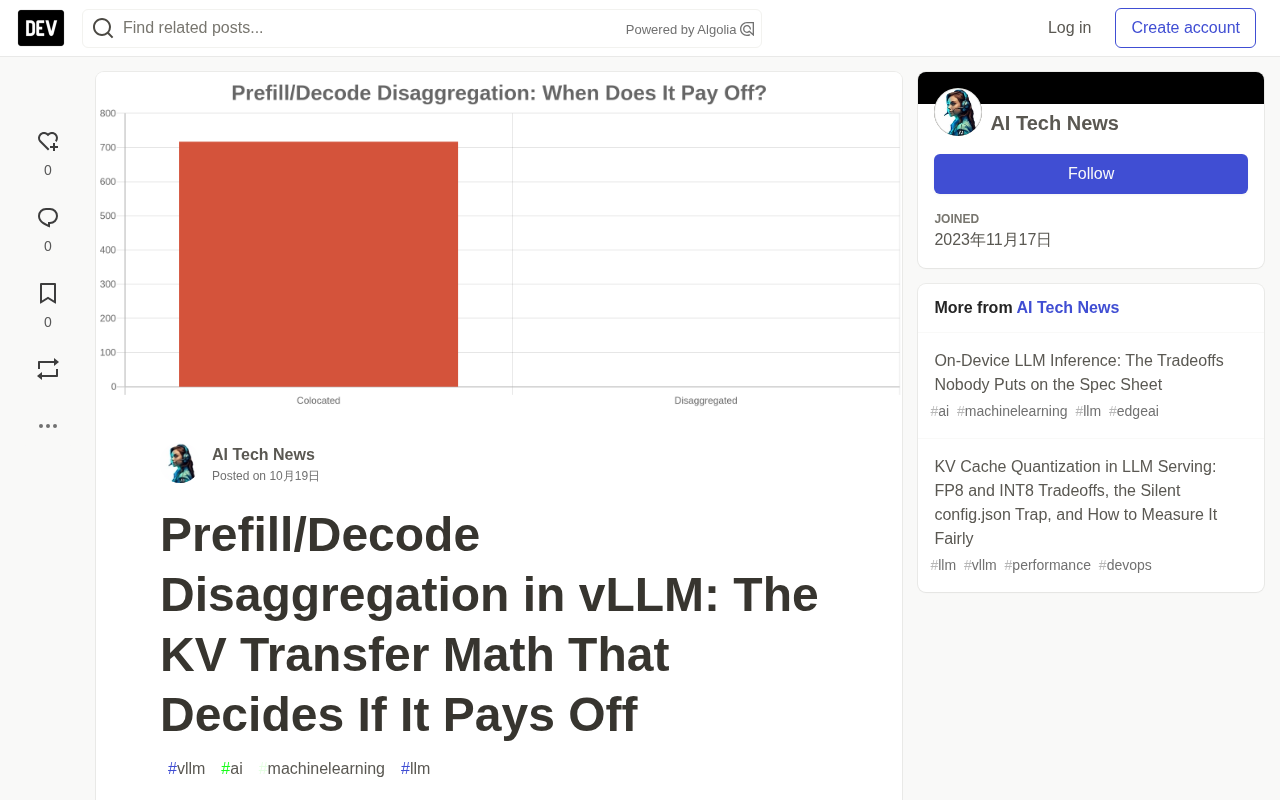
The good news is that this cost is a ratio you can compute before buying NICs. Based on public model configurations and clearly labeled assumptions, this article unpacks the arithmetic and provides an actionable decision rule.

The Hardware Personality Clash Between Prefill and Decode

To understand the value of P/D disaggregation, you first need to understand the fundamental difference between the two compute phases.

Prefill processes the entire prompt at once and is a compute-bound workload: large matrix multiplications, high arithmetic intensity, GPU tensor cores fully utilized. Decode generates only one token per step and is a memory-bandwidth-bound workload: each step must read all weights and the growing KV cache to produce a single token.

When both run on the same engine, they interfere with each other. A long prompt arriving mid-stream injects a compute-heavy step into a batch of sequences all waiting for their next token. Every sequence experiences an ITL spike roughly equal to the duration of that prefill step. What users feel is: whenever someone submits a large document, their own output stream stutters.

Chunked prefill is the common first layer of mitigation: split the prompt into chunks interleaved with decode steps, capping each pause to the chunk size. P/D disaggregation goes further: prefill runs on dedicated instances, decode instances never execute prefill steps, and the decode step rhythm becomes steady. The vLLM documentation explicitly states that this approach reduces ITL tail latency more reliably than chunked prefill.

Disaggregation also brings two secondary benefits: each phase can use its most appropriate parallelism strategy (e.g., higher tensor parallelism on the prefill side to reduce TTFT), and the two resource pools can scale independently as traffic patterns change.

Arithmetic intensity refers to the number of floating-point operations executed per byte of memory read in a computation, typically measured in FLOP/Byte. It is the core metric distinguishing compute-bound from memory-bound workloads: when arithmetic intensity is high, the GPU's compute units are the bottleneck and tensor cores can stay fully utilized; when it is low, memory bandwidth becomes the bottleneck and even abundant compute can only wait for data movement. During prefill, large matrix multiplications over the entire prompt achieve arithmetic intensity in the hundreds of FLOP/Byte, far above the GPU's bandwidth-compute balance point, making it compute-bound; during decode, each generated token requires reading all model weights and the KV cache, yielding arithmetic intensity often in the single digits, making it memory-bandwidth-bound. This difference is the fundamental reason the two phases need different parallelism strategies and hardware ratios, and the physical basis for why P/D disaggregation enables independent optimization.

The KV Transfer Arithmetic: Bytes per Token

Once prefill is moved elsewhere, the resulting KV cache must reach the decode instance before the first token can be produced. The number of bytes to transport per token is:

kv_bytes_per_token = 2 * layers * kv_heads * head_dim * dtype_bytes

The factor 2 accounts for both Key and Value. Below are shape parameters from the public config.json of two open-source models:

Model	Layers	KV Heads	Head Dim	BF16 per Token	FP8 per Token
Llama-3.1-8B	32	8	128	128 KiB	64 KiB
Llama-3.1-70B	80	8	128	320 KiB	160 KiB

What makes these numbers acceptable is Grouped Query Attention (GQA). A full multi-head attention 70B model with 64 KV heads would have 8x this KV cache.

By this calculation, an 8192-token prompt on the 70B model produces 2.68 GB of KV cache in BF16—that's the transport payload for a single request.

Grouped Query Attention (GQA), introduced by Ainslie et al. in 2023, is a compromise between multi-head attention (MHA) and multi-query attention (MQA). In standard MHA, each query head has its own independent Key and Value heads, and the KV cache grows linearly with head count; in MQA, all query heads share a single set of KV heads, minimizing cache but with noticeable quality loss. GQA divides query heads into groups, each sharing one set of KV heads—for example, Llama-3.1-70B has 64 query heads but only 8 KV heads, meaning 8 query heads share one set of KV. This reduces KV cache size and attention memory access to one-eighth of MHA with almost no quality loss. For P/D disaggregation, GQA directly determines the number of bytes that must cross the network per token, and is the key model-side factor that makes transfer cost acceptable.

The Ratio of Transfer Time to Prefill Time

The original article provides a deliberately minimal calculation script so you can substitute your own model shapes, link speeds, and measured prefill throughput.

Key assumptions must be stated clearly: 70B dense model, 4 GPUs sharing prefill, 400 TFLOPS effective compute per GPU, link running at line rate with no protocol overhead. Real prefill throughput depends on kernel implementation, tensor parallelism efficiency, and sequence length—be sure to replace eff_tflops with your own measured values.

Prompt Tokens	KV (BF16)	Prefill Time	100GbE	200Gb	400Gb
2,048	0.67 GB	179 ms	54 ms (30%)	27 ms (15%)	13 ms (7%)
8,192	2.68 GB	717 ms	215 ms (30%)	107 ms (15%)	54 ms (7%)
32,768	10.74 GB	2,867 ms	859 ms (30%)	429 ms (15%)	215 ms (7%)

Note that the percentage column is identical in every row. This is no coincidence: both transfer volume and prefill time scale linearly with prompt length, so the ratio converges to:

transfer / prefill = (kv_bytes_per_token / link_bandwidth) / (2 * params / (gpus * flops))

Prompt length cancels out. This yields several practical implications:

1. You can decide based on hardware alone. Model shape, link bandwidth, and prefill throughput determine the ratio; traffic patterns don't affect it.
2. Long prompts are actually more favorable than the table shows. Real prefill includes a superlinear-growing attention term, so compute time grows faster than transfer time for long prompts.
3. Tensor parallelism also helps the transfer side. KV heads are distributed across multiple GPUs during prefill; if each GPU has its own NIC path, aggregate bandwidth scales with the GPU group size. The 50 GB/s above refers to a single 400Gb link—per-GPU dedicated links would significantly change the conclusion, so check your topology before judging.
4. FP8 KV cache pays once and benefits twice. It halves both the memory footprint for concurrent sequences and the bytes crossing the network. If you're already doing KV cache quantization, the transfer ratio gets cheaper as a side effect.

One caveat about overlap: transfer doesn't necessarily happen serially after prefill. Implementations can begin moving earlier layers or chunks while later layers are still computing, hiding part of the cost. The numbers above represent the worst case of full wait. Overlap benefits are real but depend on connector implementation and network conditions.

How Much Does Same-Host Prefill Hurt Decode?

On the other side of the ledger is the loss you're trying to avoid. A decode step in a loaded batch is on the order of tens of milliseconds. An 8192-token prefill step under the same assumptions takes 717 ms. During that time, no sequence in the decode batch can advance.

Chunking shrinks the pause (179 ms for 2048-token chunks, 45 ms for 512-token chunks) but never eliminates it, and small chunks have their own costs: more steps per prompt, lower prefill efficiency, and longer TTFT for the chunked prompt itself. P/D disaggregation completely eliminates interference on the decode side, at the cost of adding a transfer step—equivalent to 4% to 30% of a prefill duration that no longer blocks anyone, per the table above.

So the real comparison isn't "transfer cost vs. zero cost" but transfer cost vs. the damage same-host prefill does to p99 ITL under your actual request mix. If your workload is short conversational turns, the damage is small and transfer is pure overhead. If it's long documents, long RAG contexts, or agent trajectories with large tool outputs, the damage may dominate your tail latency.

How to Configure It in vLLM

The feature is configured via --kv-transfer-config, a JSON string that selects the connector. The vLLM documentation lists connectors including NixlConnector, MooncakeConnector, LMCacheConnectorV1, and OffloadingConnector, and marks the feature as experimental with a possibly changing interface. The NixlConnector example from the docs is:

vllm serve <model> \
  --kv-transfer-config '{"kv_connector":"NixlConnector","kv_role":"kv_both","kv_buffer_device":"cuda","kv_connector_extra_config":{"backends":["UCX","GDS"]}}'

For the role values per instance, and for the router or proxy that sends prompts to prefill instances and then forwards to decode instances, consult the documentation for your installed version. This interface keeps evolving.

The direction of evolution is worth watching. A recent vLLM blog introduced a push-mode NIXL connector: in the traditional pull mode, the decode instance requests KV from the prefill instance; in push mode, the prefill instance writes KV directly into the decode instance's memory via RDMA. The goal is to remove three steps from the TTFT critical path—routing relay, decode-side memory allocation, and transfer setup. This affects the arithmetic in this article: these fixed overheads are not in the bandwidth ratio above. For small prompts, per-request setup overhead may dominate pure byte transfer time, so the ratio table is a lower bound on overhead, not an upper bound.

NIXL (NVIDIA Inference Xfer Library) is NVIDIA's open-source inference data transfer library that provides a unified abstraction layer for point-to-point KV cache movement. It doesn't implement transport itself but adapts to different hardware and protocols through pluggable backends: the UCX backend targets RDMA networks like InfiniBand and RoCE, supporting direct remote reads and writes of GPU memory; the GDS (GPUDirect Storage) backend targets direct data paths between local NVMe storage and GPUs. NIXL's value lies in decoupling connector logic from the specific interconnect, allowing vLLM's P/D disaggregated deployments to reuse the same interface across different cluster topologies. Understanding this helps interpret the backends field in --kv-transfer-config: it specifies the underlying transport channels available, and which backends to choose depends on your NIC type, driver stack, and whether GPUDirect is enabled.

How to Measure Whether It Actually Works

Don't use average latency or throughput to judge. P/D disaggregation is a tail latency tool, and the vLLM documentation explicitly says it doesn't improve throughput—throughput benchmarks will mislead you in both directions.

The right approach: continuously inject a long-prompt stream in the background while measuring p50 and p99 ITL. The client below uses the OpenAI-compatible streaming interface and records the time gap between adjacent data chunks in each response:

import asyncio, json, time, httpx

async def stream_itl(client, url, model, prompt, max_tokens=256):
    gaps, last = [], None
    body = {"model": model, "prompt": prompt, "max_tokens": max_tokens,
            "stream": True, "temperature": 0}
    async with client.stream("POST", url, json=body, timeout=300) as r:
        async for line in r.aiter_lines():
            if not line.startswith("data: ") or line.endswith("[DONE]"):
                continue
            now = time.perf_counter()
            if last is not None:
                gaps.append(now - last)
            last = now
    return gaps

Use a fixed set of short requests as "victims," start another task injecting long prompts at a constant rate, and run once each for co-located and disaggregated deployments. Report the victims' p50 and p99 ITL, plus TTFT for the long prompts.

Rules for keeping the comparison fair:

• Same total GPU count on both sides. Splitting 8 GPUs into 4 prefill + 4 decode must be compared against 8-GPU co-located, not against 4.
• Same arrival process and same prompt set, replayed from a file, not regenerated on the fly.
• Warm the prefix cache the same way before each run, or disable it entirely. A hot shared cache biases toward whichever configuration runs later, and in P/D scenarios it also changes how much KV actually needs to be transferred.
• Export and diff the final engine configs from both sides. Identical startup flags don't equal identical runtime conditions.
• Run long enough to reach steady state, and report the actual offered load, not just latency numbers.

When to Use It and When to Skip It

Scenario	Verdict
Strict p99 ITL targets, long or bursty prompts	Strong candidate
Clearly different optimal parallelism for prefill vs. decode	Strong candidate
High-speed interconnect between pools (RDMA, 200Gb+ per path)	Favorable arithmetic
Short prompts, low concurrency	Skip; chunked prefill suffices
Offline batch jobs, throughput only	Skip; no throughput gain
Only 100GbE or slower between pools, no FP8 KV	Calculate the ratio first; 30% overhead is hard to hide
Small cluster where splitting leaves both pools too small to batch effectively	Skip; utilization loss may exceed the benefit

The last row deserves emphasis. The decode pool needs enough concurrent sequences to fill batches, and the prefill pool needs enough arrival rate to stay busy. Splitting on a small cluster can leave both sides underutilized—a cost that doesn't appear in the transfer ratio at all.

FAQ

Does P/D disaggregation improve throughput? Not by itself. The vLLM documentation explicitly states that disaggregated prefill does not improve throughput. Its value is independent tuning of TTFT and ITL, plus tighter ITL tail control.

How large is the KV cache that needs to be transferred? Per token, compute 2 * layers * kv_heads * head_dim * dtype_bytes. Llama-3.1-70B in BF16 is 320 KiB per token, about 2.68 GB for an 8192-token prompt. FP8 KV halves it.

Is chunked prefill alone enough? Often yes for short prompts and moderate load. Chunking caps decode pauses to the chunk size but doesn't eliminate them. The vLLM documentation says disaggregation controls tail ITL more reliably than chunked prefill, at the cost of KV transfer and more complex deployment.

Which vLLM connector should I choose? The docs list options including NixlConnector, MooncakeConnector, LMCacheConnectorV1, and OffloadingConnector. The choice depends on your interconnect and software stack, and the feature is marked experimental—pin your version and retest after upgrades.

What's the difference between pull and push KV transfer? In pull mode, the decode instance requests KV from the prefill instance; in push mode, the prefill instance writes directly into decode memory via RDMA. The vLLM blog says this removes three steps from the TTFT critical path: routing relay, decode-side allocation, and transfer setup.

One-line Summary

P/D disaggregation is a latency engineering tool, not a throughput optimization; the ratio of KV transfer time to prefill time can be computed in advance.