LoRA Explained: Principles and Implementation of Efficient Large Model Fine-Tuning

The Core Idea Behind LoRA

LoRA (Low-Rank Adaptation) is one of the most popular methods for fine-tuning large models today. Its core innovation lies in the observation that the weight update ΔW during fine-tuning has a low-rank structure, which can be approximated by the product of two small matrices B and A.

Specifically, LoRA decomposes the large update matrix ΔW (of dimension D×D) into the product of two smaller matrices: ΔW ≈ B×A, where B has dimensions D×r and A has dimensions r×D. Here, r (the rank) is much smaller than D, so the number of parameters drops from D² to 2Dr, achieving a compression ratio of r/D. Taking D=4096 and r=8 as an example, the parameter count is only 0.39% of the original, resulting in a 250× reduction in computation.

This approach is inspired by the classical concept of low-rank approximation in linear algebra. The rank of a matrix is defined as the maximum number of linearly independent row (or column) vectors — intuitively, it represents the number of "independent information dimensions" the matrix contains. Low-rank approximation has long been widely used in data science. For example, SVD (Singular Value Decomposition) factorizes a large matrix into the product of three smaller matrices, retaining only the largest singular values to approximate the original. Collaborative filtering in recommendation systems and PCA dimensionality reduction in image compression are all applications of low-rank approximation at their core. LoRA brings this classical idea into the realm of deep learning fine-tuning, demonstrating for the first time that neural network weight updates also exhibit low-rank structure.

During training, the pretrained model weights W₀ are frozen, and only the two matrices B and A are trained. The forward propagation formula is: H = W₀X + (α/r)BAX, where α is a scaling factor that controls the magnitude of the update. At inference time, W' = W₀ + (α/r)BA can be precomputed, merging the LoRA branch directly into the original weights and achieving zero additional inference latency.

Why Does LoRA Work? The Theoretical Foundation of the Low-Rank Hypothesis

The theoretical foundation of LoRA comes from an important finding: the weight update ΔW during large model fine-tuning has an extremely low intrinsic rank. Research shows that for a 4096×4096 weight matrix, the effective information dimensionality after fine-tuning may be as low as 2, 4, or 8.

The reason behind this is that pretrained models have already learned rich, general-purpose language knowledge. Fine-tuning is not about training a new model from scratch but rather making small corrections on top of the pretrained foundation. These corrections tend to be concentrated along only a few directions. For example, when fine-tuning on a financial dataset, adjustments mainly occur in economic and financial semantic directions, while directions related to politics, military affairs, history, and other domains remain largely unchanged.

From a linear algebra perspective, the rank of a matrix represents its effective information dimensionality. Since fine-tuning involves small-magnitude, directionally concentrated corrections, there is no need for D² degrees of freedom — a low-rank matrix of rank r can effectively approximate the update. This is the mathematical principle behind LoRA's ability to achieve near full fine-tuning performance with extremely few parameters.

This low-rank hypothesis is also corroborated by research from Aghajanyan et al. in 2020, "Intrinsic Dimensionality Explains the Effectiveness of Language Model Fine-Tuning." That study showed that the fine-tuning process of pretrained language models exhibits extremely low "Intrinsic Dimensionality" — even when trainable parameters are randomly projected into a low-dimensional subspace far smaller than the original parameter space, the model can still achieve over 90% of full fine-tuning performance. This provides solid empirical support for LoRA's low-rank hypothesis.

Mathematical Formulation and Implementation Details of LoRA

Forward Propagation Formula

For any linear layer, the original forward propagation is H = W₀X. LoRA adds a parallel low-rank branch on top of this:

H = W₀X + (α/r)BAX

Where:

• W₀: Frozen pretrained weights
• B: Up-projection matrix (r×D), expanding the r-dimensional vector back to D dimensions
• A: Down-projection matrix (D×r), compressing the D-dimensional input to r dimensions
• α/r: Scaling factor, where α is a hyperparameter, divided by r to compensate for magnitude differences caused by varying ranks

The design of the scaling factor α/r is a carefully considered engineering detail. α (alpha) is a fixed hyperparameter (typically set to 16 or 32), while r is the rank. The reason for dividing α by r rather than using α directly is that when changing the size of r, the numerical scale of the BA matrix product varies with r — a larger r means more intermediate dimensions are summed, leading to larger output magnitudes. Dividing by r serves as normalization, eliminating the need to simultaneously adjust the learning rate when changing r, which greatly simplifies hyperparameter search. This design allows users to fix α first and then experiment only along the r dimension without worrying about inconsistencies in numerical scale. Microsoft's original LoRA paper recommends setting α to twice the value of r as a starting point, but in practice, α=16 or 32 performs robustly in most scenarios.

Application in Self-Attention Mechanisms

LoRA is primarily applied to the four projection matrices Q, K, V, and O in the Transformer. The Transformer is the core architecture behind virtually all modern large language models (such as GPT, LLaMA, and BERT), proposed by Vaswani et al. in the 2017 paper "Attention Is All You Need." Its central component is the self-attention mechanism: each token in the input sequence is mapped to different vector spaces through three projection matrices — Q (Query), K (Key), and V (Value) — and then attention weights are computed via dot products, with the final output obtained through weighted summation. The O (Output) matrix maps the concatenated multi-head attention results back to the original dimension. These four projection matrices (Q/K/V/O) each typically have dimensions D×D (where D is the hidden dimension) and represent the most parameter-dense parts of the Transformer, making them the primary optimization targets for LoRA.

Taking the Q matrix as an example:

Q = W_Q H + (α/r)B_Q A_Q H

where H is the hidden state. The K, V, and O matrices are handled in exactly the same way, with each projection matrix equipped with its own independent pair of B and A matrices.

Initialization Strategy

LoRA adopts the same initialization strategy as Adapter:

• Matrix A: Gaussian random initialization
• Matrix B: Zero initialization

This approach has two key advantages: First, at initialization BA=0, making the model completely equivalent to the pretrained model, so fine-tuning starts smoothly from the pretrained state. Second, keeping one matrix at zero and the other non-zero ensures effective gradient flow (if both were zero, all gradients would be zero and no updates could occur).

This initialization strategy embodies an important principle in deep learning training — symmetry breaking. If both matrices are initialized to zero, by the chain rule, ∂L/∂B contains the value of A and ∂L/∂A contains the value of B, so both gradients would be zero, and the model could never begin learning. Conversely, if both matrices are randomly initialized, the initial BA≠0 would immediately deviate from the pretrained model, potentially causing instability in the early stages of training. LoRA's "one-zero, one-random" strategy elegantly solves both problems: it guarantees stability at the training starting point while ensuring effective gradient propagation.

Choosing the Rank r

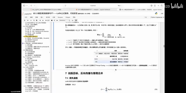
The rank r is LoRA's most important hyperparameter, controlling the model's expressive capacity and parameter count:

• At r=1, it already significantly outperforms Prompt Tuning
• At r=8, it approaches full fine-tuning performance (commonly used default)
• At r=64, it is nearly indistinguishable from full fine-tuning
• r typically ranges between 4 and 64

A larger r allows more correction directions to be combined, increasing expressive power, but also raising training costs. In practice, r=8 or 16 offers the best cost-performance tradeoff.

It's worth noting that the optimal value of r is closely related to task complexity. For simple adaptation tasks that are close to the pretraining distribution (such as general conversational style adjustment), r=4 or even r=2 may suffice. For complex tasks that require significant deviation from the pretraining distribution (such as cross-lingual transfer or cross-modal alignment), r=32 or higher may be needed. Furthermore, the optimal r may differ across layers — layers closer to the input typically carry more general features and require a smaller r, while layers closer to the output carry more task-specific information and may need a larger r. This observation has inspired follow-up work such as AdaLoRA, which adaptively assigns different ranks to different layers for further efficiency improvements.

LoRA's Advantages Over Other PEFT Methods

PEFT (Parameter-Efficient Fine-Tuning) is a family of methods designed to adapt large models using very few trainable parameters. Full Fine-Tuning requires updating all model parameters, which for models with tens or hundreds of billions of parameters means enormous memory consumption and computational costs. PEFT methods emerged to address this challenge and can be broadly categorized into three types: (1) input-side methods, such as Prompt Tuning and Prefix Tuning; (2) weight-side methods, such as Adapter and BitFit (fine-tuning only bias terms); and (3) low-rank decomposition methods, to which LoRA belongs. Each has its pros and cons, and LoRA stands out precisely because it strikes the best balance between expressive power, inference efficiency, and deployment convenience.

Comparison with Input-Side Methods (Prompt Tuning, Prefix Tuning)

Input-side methods guide the model by inserting learnable vectors at the input layer or attention layers. Prompt Tuning, proposed by Lester et al. in 2021, prepends a set of learnable "soft prompt" vectors before the input embeddings — these vectors do not correspond to any real tokens but are optimized through backpropagation. Prefix Tuning goes further by prepending learnable prefix vectors to the Key and Value at every Transformer layer, thereby injecting guidance signals at each layer. The advantages are extreme lightweight design and no modification to the model backbone, but there are three notable drawbacks:

1. Indirect expressive power: Task signals can only be conveyed through guidance, without directly modifying the feature mappings of weight matrices. This leads to poor performance on small models and complex tasks.
2. Increased sequence length: The inserted learnable vectors increase the sequence length, adding extra computational overhead during inference.
3. Deployment inconvenience: The learnable parameters exist in a different parameter space from the main model, making true parameter fusion difficult.

Comparison with Weight-Side Methods (Adapter)

The Adapter method, proposed by Houlsby et al. in 2019, inserts MLP bottleneck modules directly into Transformer layers. Specifically, the module uses a bottleneck architecture: a down-projection linear layer first compresses the D-dimensional vector to m dimensions (where m is much smaller than D), followed by a nonlinear activation function, and then an up-projection linear layer restores it to D dimensions, with a residual connection added. This adds only about 2Dm parameters per layer. While Adapter can directly modify hidden states and achieves performance close to full fine-tuning, it has two issues:

1. Increased inference latency: Information flow must pass serially through the additionally inserted MLP modules, with extra matrix multiplications and activation function computations at each layer. This introduces non-negligible latency in high-throughput inference or real-time serving scenarios.
2. Model architecture modification: It requires changing the backbone network architecture, increasing deployment complexity.

LoRA's Combined Advantages

LoRA cleverly combines the strengths of both types of methods while avoiding their respective weaknesses:

1. Direct weight modification: Through ΔW=BA, it directly updates weight matrices, providing strong expressive power.
2. Zero inference latency: At inference time, W'=W₀+(α/r)BA can be precomputed, fully merging the LoRA branch with no additional overhead.
3. Parameter efficient: The parameter count is only about 0.4% of full fine-tuning.
4. Deployment friendly: After merging, it is completely equivalent to the original model, with no changes to the inference pipeline.

To use a vivid analogy: full fine-tuning is like redrawing an entire map, while LoRA is like annotating a few key updates on the original map — preserving existing knowledge while efficiently adapting to new tasks.

Key Points of LoRA Code Implementation

A complete LoRA implementation includes the following key steps:

1. Freeze the Pretrained Model

for param in model.parameters():
    param.requires_grad = False

This step ensures that the pretrained weights W₀ remain unchanged throughout the fine-tuning process. In PyTorch, requires_grad = False means the parameter will not participate in gradient computation or optimizer updates, significantly reducing memory usage — since gradients and optimizer states (such as Adam's first and second moment estimates) do not need to be stored for these parameters. This memory savings is typically 2-3× the size of the model parameters themselves.

2. Create Low-Rank Matrices

self.lora_A = nn.Parameter(torch.randn(d, r))  # Down-projection matrix
self.lora_B = nn.Parameter(torch.zeros(r, d))  # Up-projection matrix, zero-initialized

3. Dual-Path Forward Propagation

def forward(self, x):
    # Frozen path
    y0 = F.linear(x, self.weight)  # W₀X
    # LoRA path
    lora_output = (self.alpha / self.r) * (x @ self.lora_A @ self.lora_B)
    return y0 + lora_output

4. Weight Merging (Before Deployment)

def merge_weights(self):
    self.weight.data += (self.alpha / self.r) * (self.lora_B @ self.lora_A)

Weight merging is the key step that enables LoRA's zero inference latency. After merging, the model's forward propagation path is completely identical to the original model, with no additional branch computation. In production environments, the merge operation is typically performed after fine-tuning is complete, and the merged weights are saved in standard model format for direct deployment with existing inference engines (such as vLLM or TGI). If switching between multiple LoRAs is needed (e.g., A/B testing different versions), the unmerged state can be maintained with different LoRA weights loaded dynamically at inference time — this is the foundation of multi-tenant service architectures.

5. Gradient Computation

Using the chain rule:

• ∂L/∂B = (α/r) · (∂L/∂H) · (AX)ᵀ
• ∂L/∂A = (α/r) · Bᵀ · (∂L/∂H) · Xᵀ

During training, only B and A participate in gradient updates, while W₀ remains frozen throughout.

Practical Applications and Ecosystem Development of LoRA

In industry, LoRA has become a key technology for deploying large models in production. Typical use cases include:

1. Multi-tenant services: A single base model serves different customers through different LoRA weights. Only the small LoRA parameter files (typically just tens of MB) need to be stored and swapped, eliminating the need to deploy a full model copy for each customer.

2. Image generation community: In the Stable Diffusion community, users train LoRA models with a small set of style-specific images to generate images in specific artistic styles using a general-purpose model. Platforms like Civitai host hundreds of thousands of community-contributed LoRA models, forming a thriving creator ecosystem.

3. Domain knowledge injection: Vertical domains such as healthcare, legal, and finance use LoRA fine-tuning to equip general-purpose models with specialized terminology and reasoning patterns while retaining general conversational capabilities.

4. QLoRA and extreme efficiency: QLoRA, proposed by Dettmers et al. in 2023, combines LoRA with 4-bit NormalFloat quantization, enabling fine-tuning of 65B or even 70B parameter models on a single consumer-grade GPU (such as an RTX 3090/4090 with 24GB VRAM). This dramatically lowers the hardware barrier for large model fine-tuning, enabling individual developers and small teams to participate in customized large model development.

LoRA's success has also spawned a series of follow-up improvements: DoRA (Weight-Decomposed Low-Rank Adaptation) decomposes weights into direction and magnitude components for separate adaptation; AdaLoRA adaptively assigns different ranks to different layers; and rsLoRA improves the scaling strategy to support larger rank values. Together, these works continue to drive the evolution of parameter-efficient fine-tuning techniques.

Summary

LoRA elegantly solves the parameter efficiency and inference efficiency challenges of large model fine-tuning through low-rank decomposition, establishing itself as the mainstream fine-tuning approach in the large model era. Its theoretical foundation is clear (the low-rank hypothesis), its implementation is simple (only two small matrices need to be added), its performance is excellent (near full fine-tuning results at r=8), and it can be fully merged at inference time for zero latency.

In practice, LoRA has been widely adopted for downstream task adaptation across various large models, including text generation, question answering systems, code generation, and more. Compared to other PEFT methods, LoRA demonstrates clear advantages in performance, efficiency, and ease of use, making it one of the indispensable core technologies of the large model era.

Key Takeaways